Konstantinos Patelis: Classification modelling workflow using tidymodels

Konstantinos Patelis

I was recently working through the final assignment in the Practical Machine Learning Coursera course (part of the JHU Data Science Specialization), which entailed creating a model to predict the way people perform a weight-lifting exercise using data from accelerometers on the belt, forearm, arm, and dumbell of each participant. I thought this was a good opportunity to practice using the tidymodels family of packages to tackle this classification problem. So, in this post we will go through the series of steps to create our predictive model. We will cover defining the data pre-processing, specifying the model(s) to fit and using cross-validation to tune model hyperparameters. Additionally, we’ll have a look at one of the recent additions to the tidymodels packages, stacks to create an ensemble model out of our base models. We’ll see that most of our models perform almost equally well and an ensemble model is not required for achieving improved accuracy, and is presented mostly because this was a good opportunity to try it out 😄.

Data

We’ll use the Weight Lifting Exercises data set (Velloso et al. 2013), provided as part of the Human Activity Recognition project. The data available to us is split in two parts, one is the training set, which contains the classe variable which we want to train our model to predict, and the quiz set, that contains 20 observations for which we needed to predict classe as part of the course assignment. For this blog post we’ll focus on the first data set, which we will split in two parts, one used for actually training the model and one to assess its accuracy.

## Libraries

# General data wrangling
library(tidyverse)
library(skimr)

# Modeling packages
library(tidymodels)
library(stacks)

# Visualization
library(corrr)
library(plotly)

# Parallelization
library(doParallel)

# EDA - will not be showing the outputs from using these packages, but very useful for exploration
# library(DataExplorer)
# library(explore)

theme_set(theme_bw())

## Data

initial_data <- read_data("https://d396qusza40orc.cloudfront.net/predmachlearn/pml-training.csv") %>% select(-1) # read_data is a wrapper around read_csv

EDA

Let’s split the initial data a training set and an test set (80/20 split). For the exploratory analysis and subsequent modeling, hyperparameter tuning and model evaluation I will use the training data set. Then the model will be used on the test data to predict out-of-sample accuracy.

set.seed(1992)
                            
split <- initial_split(initial_data, prop = .8, strata = classe)

train <-  training(split)
test <- testing(split)

skim(train)

Table 1: Data summary
Name	train
Number of rows	15700
Number of columns	159
_______________________
Column type frequency:
character	105
numeric	53
POSIXct	1
________________________
Group variables	None

Variable type: character

skim_variable	n_missing	complete_rate	min	max	n_unique
user_name	0	1.00	5	8	6
raw_timestamp_part_1	0	1.00	10	10	837
raw_timestamp_part_2	0	1.00	3	6	13769
new_window	0	1.00	2	3	2
kurtosis_roll_belt	15377	0.02	7	9	315
kurtosis_picth_belt	15377	0.02	7	9	258
kurtosis_yaw_belt	15377	0.02	7	7	1
skewness_roll_belt	15377	0.02	7	9	314
skewness_roll_belt.1	15377	0.02	7	9	271
skewness_yaw_belt	15377	0.02	7	7	1
max_roll_belt	15377	0.02	1	5	165
max_picth_belt	15377	0.02	1	2	22
max_yaw_belt	15377	0.02	3	7	62
min_roll_belt	15377	0.02	2	5	161
min_pitch_belt	15377	0.02	1	2	16
min_yaw_belt	15377	0.02	3	7	62
amplitude_roll_belt	15377	0.02	1	5	124
amplitude_pitch_belt	15377	0.02	1	2	13
amplitude_yaw_belt	15377	0.02	4	7	3
var_total_accel_belt	15377	0.02	1	6	60
avg_roll_belt	15377	0.02	1	8	165
stddev_roll_belt	15377	0.02	1	6	62
var_roll_belt	15377	0.02	1	7	81
avg_pitch_belt	15377	0.02	1	8	191
stddev_pitch_belt	15377	0.02	1	6	41
var_pitch_belt	15377	0.02	1	6	53
avg_yaw_belt	15377	0.02	1	8	207
stddev_yaw_belt	15377	0.02	1	6	52
var_yaw_belt	15377	0.02	1	8	122
var_accel_arm	15377	0.02	1	8	313
avg_roll_arm	15377	0.02	1	9	261
stddev_roll_arm	15377	0.02	1	8	261
var_roll_arm	15377	0.02	1	10	261
avg_pitch_arm	15377	0.02	1	8	261
stddev_pitch_arm	15377	0.02	1	7	261
var_pitch_arm	15377	0.02	1	9	261
avg_yaw_arm	15377	0.02	1	9	261
stddev_yaw_arm	15377	0.02	1	8	258
var_yaw_arm	15377	0.02	1	10	258
kurtosis_roll_arm	15377	0.02	7	8	260
kurtosis_picth_arm	15377	0.02	7	8	258
kurtosis_yaw_arm	15377	0.02	7	8	312
skewness_roll_arm	15377	0.02	7	8	261
skewness_pitch_arm	15377	0.02	7	8	258
skewness_yaw_arm	15377	0.02	7	8	312
max_roll_arm	15377	0.02	1	5	232
max_picth_arm	15377	0.02	1	5	214
max_yaw_arm	15377	0.02	1	2	49
min_roll_arm	15377	0.02	1	5	228
min_pitch_arm	15377	0.02	1	5	230
min_yaw_arm	15377	0.02	1	2	37
amplitude_roll_arm	15377	0.02	1	5	246
amplitude_pitch_arm	15377	0.02	1	6	236
amplitude_yaw_arm	15377	0.02	1	2	51
kurtosis_roll_dumbbell	15377	0.02	6	7	318
kurtosis_picth_dumbbell	15377	0.02	6	7	320
kurtosis_yaw_dumbbell	15377	0.02	7	7	1
skewness_roll_dumbbell	15377	0.02	6	7	320
skewness_pitch_dumbbell	15377	0.02	6	7	319
skewness_yaw_dumbbell	15377	0.02	7	7	1
max_roll_dumbbell	15377	0.02	1	5	282
max_picth_dumbbell	15377	0.02	2	6	285
max_yaw_dumbbell	15377	0.02	3	7	64
min_roll_dumbbell	15377	0.02	1	6	277
min_pitch_dumbbell	15377	0.02	1	6	294
min_yaw_dumbbell	15377	0.02	3	7	64
amplitude_roll_dumbbell	15377	0.02	1	6	313
amplitude_pitch_dumbbell	15377	0.02	1	6	310
amplitude_yaw_dumbbell	15377	0.02	4	7	2
var_accel_dumbbell	15377	0.02	1	7	310
avg_roll_dumbbell	15377	0.02	5	9	320
stddev_roll_dumbbell	15377	0.02	1	8	315
var_roll_dumbbell	15377	0.02	1	10	315
avg_pitch_dumbbell	15377	0.02	5	8	320
stddev_pitch_dumbbell	15377	0.02	1	7	315
var_pitch_dumbbell	15377	0.02	1	9	315
avg_yaw_dumbbell	15377	0.02	5	9	320
stddev_yaw_dumbbell	15377	0.02	1	7	315
var_yaw_dumbbell	15377	0.02	1	9	315
kurtosis_roll_forearm	15377	0.02	6	7	255
kurtosis_picth_forearm	15377	0.02	6	7	255
kurtosis_yaw_forearm	15377	0.02	7	7	1
skewness_roll_forearm	15377	0.02	6	7	256
skewness_pitch_forearm	15377	0.02	6	7	252
skewness_yaw_forearm	15377	0.02	7	7	1
max_roll_forearm	15377	0.02	1	5	224
max_picth_forearm	15377	0.02	1	5	137
max_yaw_forearm	15377	0.02	3	7	40
min_roll_forearm	15377	0.02	1	5	218
min_pitch_forearm	15377	0.02	1	5	149
min_yaw_forearm	15377	0.02	3	7	40
amplitude_roll_forearm	15377	0.02	1	5	234
amplitude_pitch_forearm	15377	0.02	1	6	154
amplitude_yaw_forearm	15377	0.02	4	7	2
var_accel_forearm	15377	0.02	1	9	319
avg_roll_forearm	15377	0.02	1	10	256
stddev_roll_forearm	15377	0.02	1	9	254
var_roll_forearm	15377	0.02	1	11	254
avg_pitch_forearm	15377	0.02	1	9	257
stddev_pitch_forearm	15377	0.02	1	8	257
var_pitch_forearm	15377	0.02	1	10	257
avg_yaw_forearm	15377	0.02	1	10	257
stddev_yaw_forearm	15377	0.02	1	9	255
var_yaw_forearm	15377	0.02	1	11	255
classe	0	1.00	1	1	5

Variable type: numeric

skim_variable	complete_rate	mean	sd	p0	p25	p50	p75	p100	hist
num_window	1	431.53	248.39	1.00	223.00	425.00	647.00	864.00	▇▇▇▇▇
roll_belt	1	64.50	62.76	-28.90	1.10	113.00	123.00	162.00	▇▁▁▅▅
pitch_belt	1	0.39	22.33	-55.80	1.79	5.31	15.20	60.30	▃▁▇▅▁
yaw_belt	1	-11.33	95.00	-180.00	-88.30	-12.95	12.53	179.00	▁▇▅▁▃
total_accel_belt	1	11.33	7.74	0.00	3.00	17.00	18.00	29.00	▇▁▂▆▁
gyros_belt_x	1	-0.01	0.20	-0.98	-0.03	0.03	0.11	2.02	▁▇▁▁▁
gyros_belt_y	1	0.04	0.08	-0.64	0.00	0.02	0.11	0.64	▁▁▇▁▁
gyros_belt_z	1	-0.13	0.24	-1.46	-0.20	-0.10	-0.02	1.62	▁▂▇▁▁
accel_belt_x	1	-5.69	29.69	-120.00	-21.00	-15.00	-5.00	85.00	▁▁▇▁▂
accel_belt_y	1	30.21	28.63	-69.00	3.00	35.00	61.00	164.00	▁▇▇▁▁
accel_belt_z	1	-72.80	100.47	-275.00	-162.00	-152.00	27.00	105.00	▁▇▁▅▃
magnet_belt_x	1	55.39	63.78	-52.00	9.00	35.00	59.00	485.00	▇▁▂▁▁
magnet_belt_y	1	593.65	35.70	354.00	581.00	601.00	610.00	673.00	▁▁▁▇▃
magnet_belt_z	1	-345.46	66.00	-621.00	-375.00	-319.00	-306.00	293.00	▁▇▁▁▁
roll_arm	1	17.52	72.88	-180.00	-32.40	0.00	77.10	180.00	▁▃▇▆▂
pitch_arm	1	-4.80	30.78	-88.20	-26.20	0.00	11.10	88.50	▁▅▇▂▁
yaw_arm	1	-0.81	71.30	-180.00	-43.12	0.00	45.10	180.00	▁▃▇▃▂
total_accel_arm	1	25.56	10.55	1.00	17.00	27.00	33.00	65.00	▃▆▇▁▁
gyros_arm_x	1	0.04	1.99	-6.37	-1.33	0.08	1.57	4.87	▁▃▇▆▂
gyros_arm_y	1	-0.26	0.85	-3.44	-0.80	-0.24	0.16	2.84	▁▂▇▂▁
gyros_arm_z	1	0.27	0.55	-2.33	-0.07	0.23	0.72	3.02	▁▂▇▂▁
accel_arm_x	1	-59.78	182.57	-404.00	-242.00	-43.00	84.00	437.00	▇▅▇▅▁
accel_arm_y	1	32.22	110.13	-318.00	-54.00	14.00	139.00	308.00	▁▃▇▇▂
accel_arm_z	1	-71.75	134.81	-629.00	-144.00	-47.00	22.00	271.00	▁▁▅▇▁
magnet_arm_x	1	192.26	443.84	-584.00	-299.00	292.00	637.00	782.00	▆▃▂▃▇
magnet_arm_y	1	155.90	201.81	-386.00	-10.00	200.00	322.00	582.00	▁▅▅▇▂
magnet_arm_z	1	305.14	327.76	-597.00	128.00	442.50	545.00	694.00	▁▂▂▃▇
roll_dumbbell	1	23.34	69.96	-152.83	-19.74	48.01	67.46	153.55	▂▂▃▇▂
pitch_dumbbell	1	-10.84	37.04	-149.59	-40.98	-20.92	17.21	137.02	▁▅▇▃▁
yaw_dumbbell	1	1.77	82.63	-150.87	-77.76	-2.45	79.65	154.95	▃▇▅▅▆
total_accel_dumbbell	1	13.68	10.22	0.00	4.00	10.00	19.00	58.00	▇▅▃▁▁
gyros_dumbbell_x	1	0.16	1.68	-204.00	-0.03	0.13	0.35	2.22	▁▁▁▁▇
gyros_dumbbell_y	1	0.05	0.64	-2.10	-0.14	0.05	0.21	52.00	▇▁▁▁▁
gyros_dumbbell_z	1	-0.12	2.55	-2.38	-0.31	-0.13	0.03	317.00	▇▁▁▁▁
accel_dumbbell_x	1	-28.70	67.30	-419.00	-50.00	-8.00	11.00	235.00	▁▁▆▇▁
accel_dumbbell_y	1	52.08	80.40	-189.00	-9.00	41.00	110.00	315.00	▁▇▇▅▁
accel_dumbbell_z	1	-38.29	109.45	-334.00	-142.00	-1.00	38.00	318.00	▁▆▇▃▁
magnet_dumbbell_x	1	-329.02	339.83	-643.00	-535.00	-480.00	-307.00	592.00	▇▂▁▁▂
magnet_dumbbell_y	1	220.31	327.15	-3600.00	231.00	310.00	390.00	633.00	▁▁▁▁▇
magnet_dumbbell_z	1	45.46	139.97	-262.00	-46.00	12.00	95.00	452.00	▁▇▆▂▂
roll_forearm	1	33.46	108.15	-180.00	-1.11	21.10	140.00	180.00	▃▂▇▂▇
pitch_forearm	1	10.74	28.10	-72.50	0.00	9.39	28.40	89.80	▁▁▇▃▁
yaw_forearm	1	19.16	103.19	-180.00	-68.50	0.00	110.00	180.00	▅▅▇▆▇
total_accel_forearm	1	34.65	10.07	0.00	29.00	36.00	41.00	108.00	▁▇▂▁▁
gyros_forearm_x	1	0.16	0.65	-22.00	-0.22	0.05	0.56	3.26	▁▁▁▁▇
gyros_forearm_y	1	0.07	3.29	-6.65	-1.48	0.03	1.62	311.00	▇▁▁▁▁
gyros_forearm_z	1	0.15	1.94	-7.94	-0.18	0.08	0.49	231.00	▇▁▁▁▁
accel_forearm_x	1	-62.00	180.67	-498.00	-179.00	-57.00	77.00	477.00	▂▆▇▅▁
accel_forearm_y	1	163.38	199.43	-632.00	57.75	200.00	312.00	923.00	▁▂▇▅▁
accel_forearm_z	1	-54.90	138.27	-446.00	-181.00	-38.00	26.00	291.00	▁▇▅▅▃
magnet_forearm_x	1	-312.71	346.77	-1280.00	-616.00	-379.00	-74.00	672.00	▁▇▇▅▁
magnet_forearm_y	1	379.89	508.80	-896.00	2.00	593.00	737.00	1480.00	▂▂▂▇▁
magnet_forearm_z	1	394.70	368.72	-973.00	192.75	512.00	653.00	1090.00	▁▁▂▇▃

Variable type: POSIXct

skim_variable	n_missing	complete_rate	min	max	median	n_unique
cvtd_timestamp	0	1	2011-11-28 14:13:00	2011-12-05 14:24:00	2011-12-02 13:35:00	20

It seems like the majority of the variables are numeric, but one important thing to note is that there is a high percentage of missing observations for a subset of the variables. From the completion rate, it seems that the missing values across the different attributes occur for the same observations. Since the majority of observations have missing values for these variables, it is unlikely that we could impute them. When viewing the data in spreadsheet applications these variables have a mix of being coded as NA or being simply blank, while even for observations where values are available, there are instances of a value showing as #DIV/0.

eda <- train %>% select(where(~ !any(is.na(.))))

One important thing in classification problems is to investigate whether there is imbalance between the different classes in our training data. For example, if a class is over-represented in the data then our classifier might tend to over-predict that class. Let’s check how many times each class appears in the data.

ggplot(eda, aes(classe, fill = classe)) + 
  geom_bar() + 
  theme_bw()

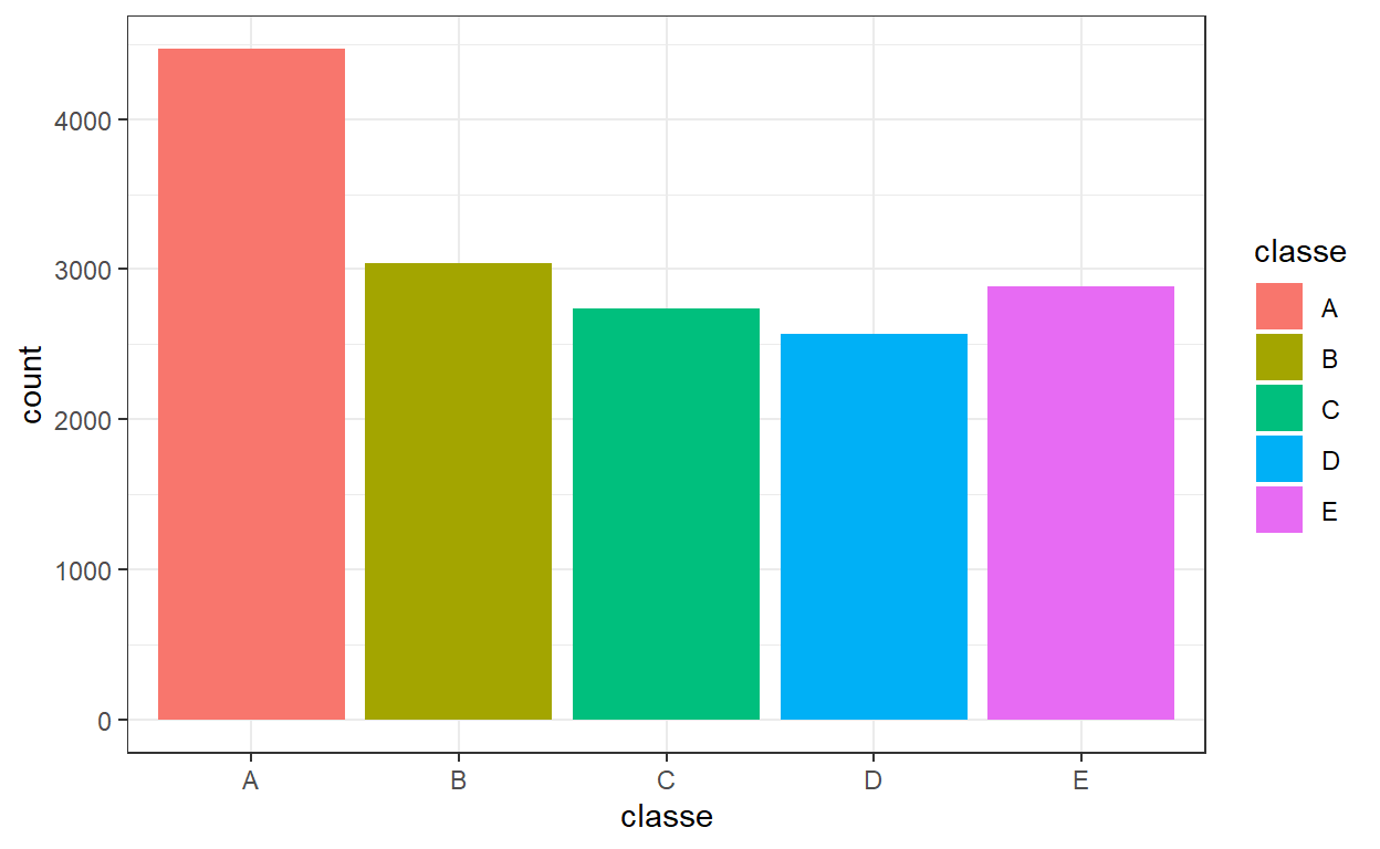
Looking at the above, there does not seem to be severe imbalance among classes. We can also use a normalised version of the Shannon diversity index to understand how balanced our data set is. A value of 0 would indicate an unbalanced data set and a value of 1 would point to the data being balanced.

balance <- train %>% 
  group_by(classe) %>% 
  count() %>% 
  ungroup() %>% 
  mutate(check = - (n / sum(n) * log(n / sum(n))) / log(length(classe)) ) %>% 
  summarise(balance = sum(check)) %>% 
  pull()

balance

[1] 0.9865199

A value of 0.9865199 indicates we don’t have an imbalance issue.

Considering the other columns in our data, user name cannot be part of our predictors because it cannot generalize to other data if our model was used on data that is not part of this study. Looking at the timestamp, each subject was fully measured at a different point in the day, with each exercise happening back-to-back. From Velloso et al. (2013) (Velloso et al. 2013), we know that all subjects were observed in the presence of a professional trainer to observe that the exercise was done according to specification each time. I will not consider the timestamps or any features derived from them (e.g. using the time of day) as a predictor in our models.

eda %>% 
  mutate(new_window = as.numeric(factor(new_window))) %>% 
  select(where(is.numeric)) %>% 
  correlate(method = "pearson", quiet = TRUE) %>% 
  shave() %>% 
  rplot() %>% 
  ggplotly()

Even excluding the columns mentioned above, there are a lot of features and presenting more information on EDA here would get too extensive. Since the purpose here is to demonstrate the modeling process with tidymodels, we will not be performing a more extensive EDA. For quick data exploration, you can use DataExplorer::create_report(eda) and explore::explore(eda) (after installing the two packages) to get a full data report on the data set from the former and a shiny app for interactive exploration from the latter.

Modelling

In this section we will define the recipe to pre-process the data, specify the models and combine these steps in a workflow. Then we will use cross-validation to tune the various hyper-parameters of the models.

Pre-processing Recipe

I will use the recipes package to provide a specification of all the transformations to the data set before I fit any models, which will ensure that the same transformations are applied to the training, test and quiz data in the same way. Furthermore, it helps avoid information leakage as the transformations will be applied to all data sets using the statistics calculated for the training data. Specifically, I will remove all variables with missing values as well as other attributes discussed above, perform a transformation to try to make all predictors more symmetric (which is useful for models that benefit from predictors with distributions close to the Gaussian), normalize all variables (particularly important for the KNN and glmnet models) and then removing any predictors, if any, with very small variance. Note that we could define different pre-processing steps if required by the various models we will be tuning.

# Creating a vector with the names of all variables that should be removed because they contain NAs

cols_rm <- train %>% 
  select(where(~ any(is.na(.)))) %>% 
  colnames()

model_recipe <- recipe(classe ~ ., data = train) %>% 
  step_rm(all_of(!!cols_rm), all_nominal(), -all_outcomes(), 
          cvtd_timestamp, num_window, 
          new_window) %>% 
  step_YeoJohnson(all_predictors()) %>% 
  step_normalize(all_predictors()) %>% 
  step_nzv(all_predictors())

# Below rows can be used to perform the transformation on the training set. Since we will be using the workflow package, this is not required.

# model_recipe_prepped <- model_recipe %>% prep()
# baked_recipe <- model_recipe_prepped %>% bake(new_data = NULL)

Model Specification

In this section I will use the parsnip package to create model specifications and set which model parameters will need to be tuned to ensure higher model performance. I will be trying four different models:

Random Forests (rf) - with 1000 trees and we will tune the number of predictors at each node split and the minimum number of data points in a node required for the node to be further split.
K Nearest Neighbours (knn) - with a tunable number k of neighbours, kernel function with which to weight distances, and the parameter for the Minkowski distance.
Multinomial Logistic Regression with Regularization (lm) - with a tunable regularization penalty.
Boosted Trees (boost) - where we tune the number of trees, the learning rate, tree depth, number of predictors at each node split and the minimum number of data points in a node.

I will then use the workflows package to combine the model recipe and the model specifications into different workflows. With parsnip we can create the specification in a similar manner across models and specify “computational engines” - practically R functions/packages that implement the calculations.

rf_model <- rand_forest(
                        mtry = tune(),
                        min_n = tune(),
                        trees = 1000
                        ) %>% 
            set_mode("classification") %>% 
            set_engine("ranger")
            

# rf_fit <- fit(rf_model, classe ~ ., data = baked_recipe) # This call could be used to fit the model to the training data, but we will be using the workflows interface

knn_model <- nearest_neighbor(
                              neighbors = tune(), 
                              weight_func = tune(), 
                              dist_power = tune()
                              ) %>% 
             set_engine("kknn") %>% 
             set_mode("classification")

# knn_fit <- fit(knn_model, classe ~ ., data = baked_recipe)

lasso_model <- multinom_reg(
                             penalty = tune(),
                             mixture = 1
                             ) %>% 
                set_engine("glmnet")

# lasso_fit <- fit(lasso_model, classe ~ ., data = baked_recipe)

boost_model <- boost_tree(
                          trees = tune(), 
                          mtry = tune(),
                          min_n = tune(),
                          learn_rate = tune(),
                          tree_depth = tune()
                          ) %>% 
               set_engine("xgboost") %>% 
               set_mode("classification")

# boost_fit <- fit(boost_model, classe ~ ., data = baked_recipe)

# Combine the model and the pre-processing recipe in a workflow (per each model)

rf_wf <- workflow() %>% 
  add_model(rf_model) %>% 
  add_recipe(model_recipe)

knn_wf <- workflow() %>% 
  add_model(knn_model) %>% 
  add_recipe(model_recipe)

lasso_wf <- workflow() %>% 
  add_model(lasso_model) %>% 
  add_recipe(model_recipe)

boost_wf <- workflow() %>% 
  add_model(boost_model) %>% 
  add_recipe(model_recipe)

Model Tuning

Let us tune the different model parameters using 10-fold cross-validation. To create the grid with the combinations of parameters we can use a space-filling design with 30 points, based on which 30 combinations of the parameters will be picked such that they cover the most area in the design space. The dials package contains sensible default ranges for the most common hyperparameters that are tuned in models. The user can modify those if required, and for some, the default range depends on the number of features. One such example is the mtry parameter in random forests and boosted trees algorithms, whose max value is equal to the number of predictors in the processed data set. If the number of predictors is known, we can use the finalize function to assign the range for mtry. This would not be possible if our model recipe contained steps that tune the final number of predictors (e.g. pre-processing with PCA and tuning the number of components to keep).

# Extract the parameters that require tuning to pass into the tuning grid

trained_data <- model_recipe %>% prep() %>% bake(new_data = NULL)

rf_param <- parameters(rf_wf) %>% finalize(trained_data)
knn_param <- parameters(knn_wf) 
lasso_param <- parameters(lasso_wf)
boost_param <- parameters(boost_wf) %>% finalize(trained_data)

rf_param %>% pull_dials_object("mtry")

# Randomly Selected Predictors (quantitative)
Range: [1, 53]

When tuning a model, it is always important to consider what we are trying to optimize the model (e.g. achieve highest possible accuracy, maximize true positives, etc). For our problem, the aim is to accurately predict the class of each observation, so at the end of the tuning process we will pick the hyperparameters that achieve highest accuracy. When tuning classification models with the tune package, by default the accuracy and area under the ROC curve are calculated for each fold. We can specify other metrics from the yardstick package to calculate while tuning by specifying the metrics parameter e.g. in tune_grid. Note that if the metrics specified perform hard class predictions (if we selected accuracy as our sole metric), then classification probabilities are not created. Since these are required for our ensemble model in a later section, we’ll also calculate the area under the curve to get the probabilities.

# Split the train set into folds

set.seed(9876)

folds <- vfold_cv(data = train, v = 10, strata = "classe")

# requires the doParallel package to fit resamples in parallel

cl <- makePSOCKcluster(10) # select the number of cores to parallelize the calcs across
registerDoParallel(cl)

set.seed(753)

rf_tune <- rf_wf %>%
  tune_grid(
    folds,
    grid = 30,
    param_info = rf_param,
    control = control_grid(
      verbose = TRUE,
      allow_par = TRUE,
      save_pred = TRUE,
      save_workflow = TRUE,
      parallel_over = "resamples"
    )
  )

# 3423.57 sec elapsed

set.seed(456)

knn_tune <- knn_wf %>%
  tune_grid(
    folds,
    grid = 30,
    param_info = knn_param,
    control = control_grid(
      verbose = TRUE,
      allow_par = TRUE,
      save_pred = TRUE,
      save_workflow = TRUE,
      parallel_over = "resamples"
    )
  )

# 8419.63 sec elapsed

lasso_tune <- lasso_wf %>%
  tune_grid(
    folds,
    grid = 30,
    param_info = lasso_param,
    control = control_grid(
      verbose = TRUE,
      allow_par = TRUE,
      save_pred = TRUE,
      save_workflow = TRUE,
      parallel_over = "resamples"
    )
  )

set.seed(1821)

boost_tune <- boost_wf %>%
  tune_grid(
    folds,
    grid = 30,
    param_info = boost_param,
    control = control_grid(
      verbose = TRUE,
      allow_par = TRUE,
      save_pred = TRUE,
      save_workflow = TRUE,
      parallel_over = "resamples"
    )
  )

stopCluster(cl)

In-sample Accuracy

One can use the collect_metrics() function to each of these to visualize the average accuracy for each combination of parameters (averaging across resamples), and see the various hyperparameters that achieve such accuracy.

autoplot(rf_tune, metric = "accuracy")

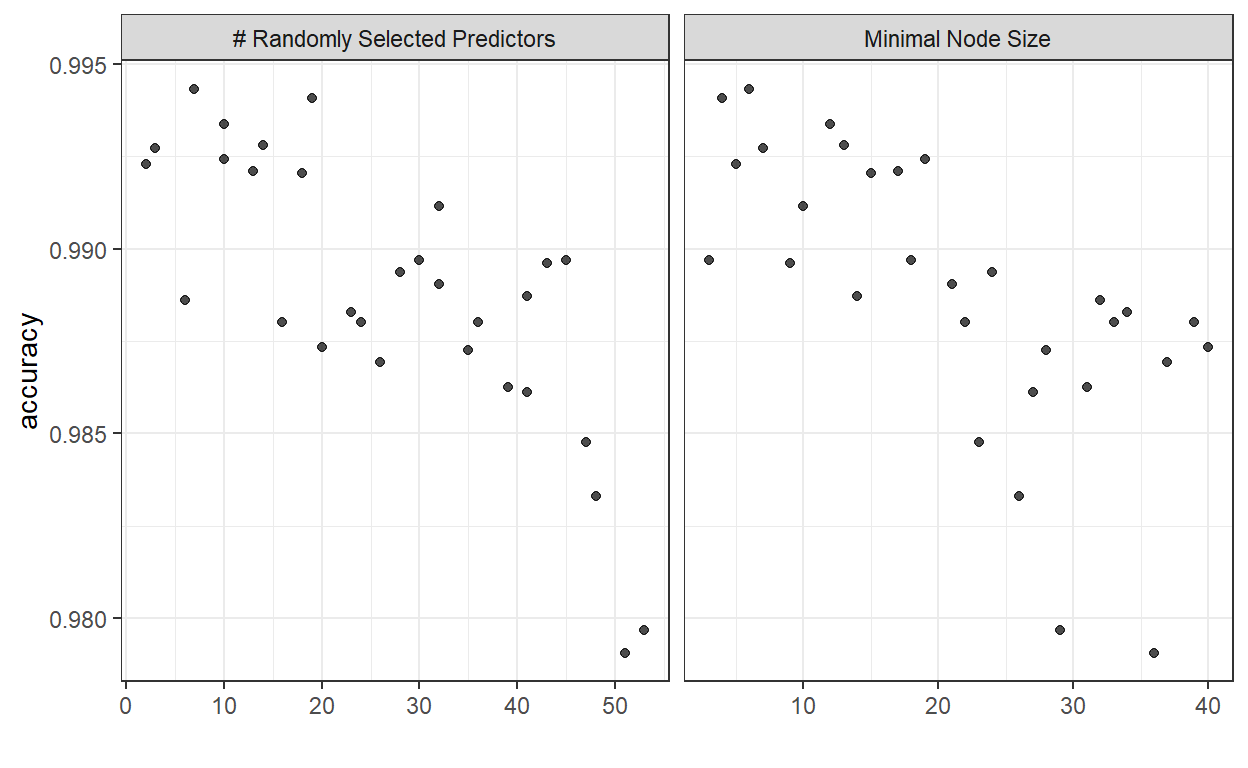
We can see that for the random forests model a combination of around 15-20 predictors and a minimal node size in the range between 5-15 seem to be optimal.

autoplot(knn_tune, metric = "accuracy")

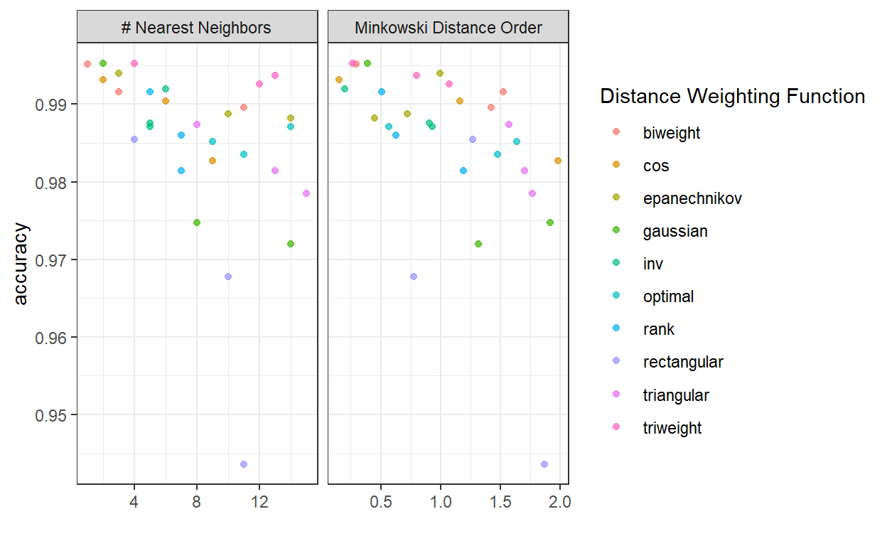
For K-NN, a small number of neighbours is preferred, while Minkowski Distance of order 0.25 seems to perform best.

autoplot(lasso_tune, metric = "accuracy")

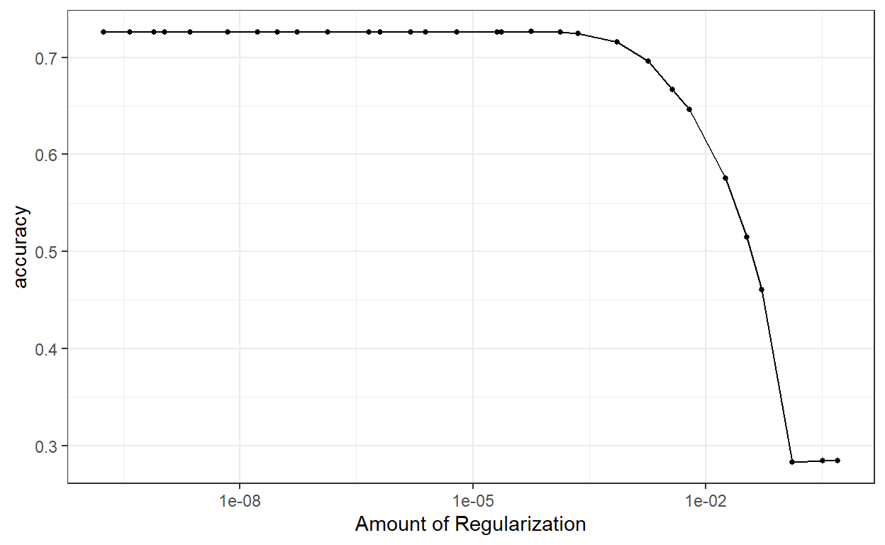
Small penalty is preferred for the LASSO model and it seems that up to a point, similar accuracy levels are achieved.

autoplot(boost_tune, metric = "accuracy")

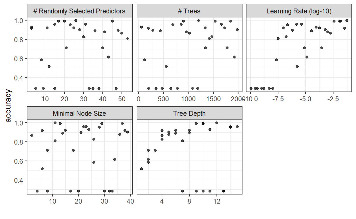
For boosted trees, it seems that a higher learning rate is better. Higher tree depth (especially in the range of 9-14) seems to provide best results, while the number of trees and the minimal node size seem to have a wide range of values for which we achieve increased accuracy.

Let us select the best models from each type of model and compare in-sample accuracy.

best_resamples <- 
  bind_rows(
            show_best(rf_tune, metric = "accuracy", n = 1) %>% mutate(model = "Random Forest") %>% select(model, accuracy = mean),  
            show_best(knn_tune, metric = "accuracy", n = 1) %>% mutate(model = "K-NN") %>% select(model, accuracy = mean), 
            show_best(lasso_tune, metric = "accuracy", n = 1) %>% mutate(model = "Logistic Reg") %>% select(model, accuracy = mean), 
            show_best(boost_tune, metric = "accuracy", n = 1) %>% mutate(model = "Boosted Trees") %>% select(model, accuracy = mean)
  )

best_resamples %>% 
  arrange(desc(accuracy)) %>% 
  knitr::kable()

model	accuracy
Boosted Trees	0.9960509
K-NN	0.9952871
Random Forest	0.9943320
Logistic Reg	0.7265596

We can see that the random forests, K-NN, and boosted trees models perform exceptionally on the resamples of the train data, while even the best lasso logistic regression model performs much worse than the other three. However, there is high chance that our models have overfit on the training data and actually will not perform as well when generalizing to new data. This is where out-of-sample data comes to play, as we will use the portion of the data we set aside at the beginning to calculate accuracy on new data.

Out-of-sample Accuracy

Now that we have a set of hyperparameters that optimize performance for each model, we can update our workflows, fit them on the entirety of the training set and perform predictions on the test set. Since the test set is part of our initial data set that we set aside, the classe variable is known and thus we can calculate accuracy. The LASSO logistic regression model probably will not be useful for prediction but for completeness I will calculate test set accuracy for all models.

# Final Random Forests Workflow

rf_best_accuracy <- select_best(rf_tune, metric = "accuracy") # retain the values of the hyperparameters that optimize accuracy
rf_wf_final <- finalize_workflow(rf_wf, rf_best_accuracy) # and pass them on to the workflow

set.seed(1209)

rf_final_fit <- last_fit(rf_wf_final, split) # use last_fit with the split object created at the start to fit the model on the training set and predict on the test set

# Final KNN

knn_best_accuracy <- select_best(knn_tune, metric = "accuracy")
knn_wf_final <- finalize_workflow(knn_wf, knn_best_accuracy)

set.seed(1387)

knn_final_fit <- last_fit(knn_wf_final, split) 

# LASSO

lasso_best_accuracy <- select_best(lasso_tune, metric = "accuracy")
lasso_wf_final <- finalize_workflow(lasso_wf, lasso_best_accuracy)
lasso_final_fit <- last_fit(lasso_wf_final, split) 

# Final Boosted Tree

boost_best_accuracy <- select_best(boost_tune, metric = "accuracy")
boost_wf_final <- finalize_workflow(boost_wf, boost_best_accuracy)

set.seed(54678)

boost_final_fit <- last_fit(boost_wf_final, split)

best_oos <- bind_rows(
                      rf_final_fit %>% mutate(model = "Random Forest"), 
                      knn_final_fit %>% mutate(model = "K-NN"), 
                      lasso_final_fit %>% mutate(model = "LASSO LogReg"), 
                      boost_final_fit %>% mutate(model = "Boosted Trees")
                      ) %>% 
  select(model, .metrics) %>% 
  unnest(cols = .metrics) %>% 
  filter(.metric == "accuracy") %>% 
  arrange(desc(.estimate))

best_oos %>% knitr::kable()

model	.metric	.estimator	.estimate	.config
Boosted Trees	accuracy	multiclass	0.9982152	Preprocessor1_Model1
K-NN	accuracy	multiclass	0.9961754	Preprocessor1_Model1
Random Forest	accuracy	multiclass	0.9943906	Preprocessor1_Model1
LASSO LogReg	accuracy	multiclass	0.7376339	Preprocessor1_Model1

We can see that the boosted trees and k nearest neighbours models perform the great, with random forest trailing slightly behind. The LASSO logistic regression model has much lower performance and would not be preferred. At this point we could walk away with a model that has a 99.8% accuracy on unseen data. However, we can take it a couple of steps further to see if we can achieve even greater accuracy, as we’ll see in the next sections.

Ensemble Model

In the previous section we used the tune package to try out different hyperparameter combinations over our data and estimate model accuracy using cross-validation. Let’s assume we haven’t yet tested the best model on our test data as we’re only supposed to use the test set for final selection and we shouldn’t be using the knowledge from applying to test data to improve performance. We can use the objects that were created with tune_grid to add the different model definitions to the model stack. Remember when we specified in the arguments that we save the predictions and workflows? This is because this information is required for this step, to combine the different models. Furthermore, the reason why we kept roc_auc as a metric while tuning is because it creates soft predictions, which are required in classification problems to create the stack. Since the outputs of these models will be highly correlated, the blend_predictions function performs regularization to decide which outputs will be used in the final prediction.

# cl <- makePSOCKcluster(5)
# registerDoParallel(cl)

set.seed(5523)

model_stack <- stacks() %>% 
  add_candidates(rf_tune) %>% 
  add_candidates(knn_tune) %>%
  add_candidates(lasso_tune) %>%
  add_candidates(boost_tune) %>% 
  blend_predictions(metric = metric_set(accuracy))

model_stack_fit <- model_stack %>% fit_members()

# stack_pred_train <- train %>% 
#   bind_cols(., predict(model_stack_fit, new_data = ., type = "class"))

stack_pred_test <- test %>% 
  bind_cols(., predict(model_stack_fit, new_data = ., type = "class"))

# stopCluster(cl)

# stack_pred_train %>% accuracy(factor(classe), .pred_class)
stack_pred_test %>% 
  accuracy(factor(classe), .pred_class) %>% 
  knitr::kable()

.metric	.estimator	.estimate
accuracy	multiclass	0.9982152

We see that in the end we achieved the same accuracy as our best model, which is not unexpected considering our accuracy was almost perfect. We can also have a look at the weights of the different models used in the ensemble.

autoplot(model_stack_fit, type = "weights") %>% 
  ggplotly()

While there was not much room for improvement, as mentioned in the beginning, this was a good opportunity to play around with the new package in practice.

Although this data set did not present much of a challenge in terms of predicting the outcome, we managed to cover many of the different steps in the modelling process using tidymodels. Further steps one could take in their analyses could potentially involve using functionality from the tidyposterior package to make statistical comparisons between the models we constructed that performed similarly. Finally, the tidymodels ecosystem of packages is constantly growing and as an example, parts of this process could be further simplified/combined using the new workflowsets package which became available on CRAN while I was working on this post.

Velloso, Eduardo, Andreas Bulling, Hans Gellersen, Wallace Ugulino, and Hugo Fuks. 2013. “The 4th Augmented Human International Conference.” In. ACM Press. https://doi.org/10.1145/2459236.2459256.

Classification modelling workflow using tidymodels

Data

EDA

Modelling

Pre-processing Recipe

Model Specification

Model Tuning

In-sample Accuracy

Out-of-sample Accuracy

Ensemble Model

References

Citation